Molecular dynamics: depinning under applied force and torque
This notebook drives a rigid cluster with an applied external force \(F_x\) or torque \(\tau_\text{ext}\) and finds the depinning transition: the critical force \(F_c\) (or critical torque \(\tau_c\)) above which the cluster begins to slide.
The dynamics follow the overdamped Langevin (Euler–Maruyama) equations:
where \(\eta_t\) and \(\eta_r\) are the translational and rotational drag coefficients (computed from \(N\) and the moment of inertia), and the noise satisfies the fluctuation-dissipation theorem:
sweep_md runs one MD trajectory per grid point (here: per \(F_x\) or \(\tau\) value) in parallel, then applies a post-processing function to extract a scalar metric (drift velocity or angular velocity). The depinning appears as a sharp onset in that metric.
[1]:
import numpy as np
from numpy import sqrt
import matplotlib.pyplot as plt
from time import time

from flake.substrate import substrate_from_params, get_ks
from flake.cluster import cluster_from_params, calc_cluster_langevin
from flake.dynamics import run_md
from flake.sweep import sweep_md, grid_sweep, drift_velocity, mean_velocity
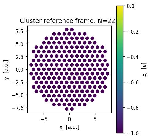
System definition
Commensurate cluster on a sinusoidal triangular substrate (\(\rho = 1\)). You can setup the same geometry as the barrier notebook so the depinning force \(F_c\) is directly comparable to the static friction \(F_s\) computed from the MEP.
kBT = 1e-8 instead of 0 avoids saddle-point ambiguity in the Euler–Maruyama integrator. At \(\epsilon = 1\) this is thermally negligible (effectively \(T = 0\)).
[2]:
ks = get_ks(1, 3, 4./3., 0.)   # triangular substrate wave vectors

params = {
    'sub_basis':     [[0, 0]],
    'epsilon':       1,
    'well_shape':    'sin',
    'ks':            ks,
    'a1':            np.array([1.,  0.]),
    'a2':            np.array([0.5, -sqrt(3.)/2.]),
    'cl_basis':      [[0, 0]],
    'cluster_shape': 'circle',
    'N1': 15, 'N2': 15,
    'theta': 0.0, 'pos_cm': [0., 0.],
}

pen_func, en_func, en_inputs = substrate_from_params(params)
pos = cluster_from_params(params)
N   = pos.shape[0]

# Translational and rotational drag coefficients.
# eta_r / eta_t ~ <r^2> / 1 sets the ratio of rotational to translational
# relaxation times -- larger clusters relax rotationally more slowly.
eta = 1.0
eta_t, eta_r = calc_cluster_langevin(eta, pos)
pen = pen_func(pos + params['pos_cm'], params['pos_cm'], *en_inputs)[0]
print('N=%i  E=%.3g  eta_t=%.3g  eta_r=%.3g  eta_r/eta_t=%.3g'
      % (N, np.sum(pen), eta_t, eta_r, eta_r/eta_t))

fig, ax = plt.subplots(dpi=120, figsize=(4, 4))
sc = ax.scatter(pos[:, 0], pos[:, 1], c=pen, vmin=-params['epsilon'], vmax=0)
plt.colorbar(sc, ax=ax, label=r'$E_i$  [$\epsilon$]')
ax.set_xlabel('x  [a.u.]')
ax.set_ylabel('y  [a.u.]')
ax.set_title('Cluster reference frame, N=%d' % N)
ax.set_aspect('equal')
plt.tight_layout()
plt.show()
N=223 E=-223 eta_t=223 eta_r=6.86e+03 eta_r/eta_t=30.8
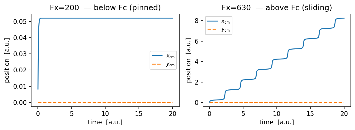
Single trajectory: below and above depinning
Before running the full sweep it is instructive to watch individual trajectories at \(F_x\) just below and just above the depinning threshold. This gives physical intuition for what the sweep is measuring: - Pinned (\(F_x < F_c\)): the CM is stuck at fixed point. - Sliding (\(F_x > F_c\)): the CM drifts with a finite average velocity.
[3]:
base_kw = dict(
    eta=1.0, kBT=1e-8, dt=1e-3, n_steps=20000,
    Tau=0., print_every=10,
    pos_cm0=params['pos_cm'],
)

fig, axes = plt.subplots(1, 2, dpi=150, figsize=(8, 3))
for ax, Fx_test, label in [
    (axes[0], 200.,  'below Fc (pinned)'),
    (axes[1], 630.,  'above Fc (sliding)'),
]:
    traj = run_md(pos, en_func, en_inputs, Fx=Fx_test, **base_kw)
    t, xcm, ycm = traj['t'], traj['pos_cm'][:, 0], traj['pos_cm'][:, 1]
    ax.plot(t, xcm, label=r'$x_\mathrm{cm}$')
    ax.plot(t, ycm, label=r'$y_\mathrm{cm}$', ls='--')
    ax.set_xlabel('time  [a.u.]')
    ax.set_ylabel('position  [a.u.]')
    ax.set_title('Fx=%.0f  — %s' % (Fx_test, label))
    ax.legend(fontsize=8)
plt.tight_layout()
plt.show()
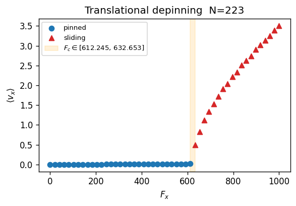
## Force sweep: translational depinning
grid_sweep({'Fx': ...}) generates one parameter set per \(F_x\) value. drift_velocity() post-processes each trajectory to extract \(\langle v_x \rangle = (x_f - x_0)/(t_f - t_0)\) — a scalar that is \(\approx 0\) in the pinned state and grows linearly above depinning.
n_jobs=-1 uses all available CPUs; each trajectory is independent.
[4]:
t0 = time()

spec = grid_sweep({'Fx': np.linspace(0., 1000., 50)})

results = sweep_md(
    pos, en_func, en_inputs, spec,
    base_md_kwargs={
        'eta':         1.0,
        'kBT':         1e-8,
        'dt':          1e-3,
        'n_steps':     10000,
        'Tau':         0.,
        'print_every': 10,
        'pos_cm0':     params['pos_cm'],
    },
    post_fn=drift_velocity(),
    n_jobs=-1,
    save=False,
    verbose=False,
)

Fx_vals = np.array([r['params']['Fx'] for r in results])
vdrift  = np.array([r['result']       for r in results])

print('Done: %.1fmin' % ((time() - t0) / 60.))
Done: 0.2min
The depinning transition appears as a sharp onset in drift velocity.
Pinned (\(F_x < F_c\)): \(\langle v_x \rangle \approx 0\)
Sliding (\(F_x > F_c\)): \(\langle v_x \rangle\) grows linearly with \(F_x - F_c\)
The orange band brackets the transition region \([F_c^\text{lo},\, F_c^\text{hi}]\). The threshold 1e-1 is appropriate in this coarse example because kBT=1e-8, so thermal drift is negligible — any \(v_x > 10^{-2}\) is genuine sliding.
[5]:
fig, ax = plt.subplots(dpi=120, figsize=(5, 3.5))

pinned  = vdrift[:, 0] < 1e-1
sliding = ~pinned

ax.scatter(Fx_vals[pinned],  vdrift[pinned,  0], color='tab:blue',
           label='pinned', zorder=3)
ax.scatter(Fx_vals[sliding], vdrift[sliding, 0], color='tab:red',
           marker='^', label='sliding', zorder=3)

if sliding.any() and pinned.any():
    Fc_lo = Fx_vals[pinned].max()
    Fc_hi = Fx_vals[sliding].min()
    ax.axvspan(Fc_lo, Fc_hi, alpha=0.15, color='orange',
               label=r'$F_c \in [%.3f,\, %.3f]$' % (Fc_lo, Fc_hi))

ax.set_xlabel(r'$F_x$')
ax.set_ylabel(r'$\langle v_x \rangle$')
ax.legend(fontsize=8)
ax.set_title('Translational depinning  N=%i' % N)
plt.tight_layout()
plt.show()
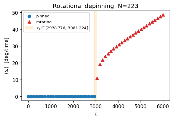
Torque sweep: rotational depinning
Same idea, but driving the cluster with an applied torque \(\tau_\text{ext}\) instead of \(F_x\). drift_omega extracts \(\langle \omega \rangle = (\theta_f - \theta_0)/(t_f - t_0)\), the angular drift velocity. A sharp onset in \(\langle \omega \rangle\) marks the rotational depinning threshold \(\tau_c\).
[6]:
def drift_omega():
    """Post-processing: return angular drift velocity dtheta/dt in deg/time."""
    def _post_fn(traj_dict, run_params):
        theta  = traj_dict['theta']
        t      = traj_dict['t']
        dt_tot = float(t[-1] - t[0])
        if dt_tot == 0.:
            return 0.
        return (theta[-1] - theta[0]) / dt_tot
    return _post_fn


t0 = time()

spec_tau = grid_sweep({'Tau': np.linspace(0., 6000., 50)})

results_tau = sweep_md(
    pos, en_func, en_inputs, spec_tau,
    base_md_kwargs={
        'eta':         1.0,
        'kBT':         1e-8,
        'dt':          1e-3,
        'n_steps':     50000,
        'print_every': 10,
    },
    post_fn=drift_omega(),
    n_jobs=-1,
    save=False,
    verbose=False,
)

Tau_vals = np.array([r['params']['Tau'] for r in results_tau])
odrift   = np.array([r['result']        for r in results_tau])

print('Done: %.1fmin' % ((time() - t0) / 60.))
Done: 0.2min
[7]:
fig, ax = plt.subplots(dpi=120, figsize=(5, 3.5))

pinned   = odrift < 1e-1
rotating = ~pinned

ax.scatter(Tau_vals[pinned],   odrift[pinned],   color='tab:blue',
           label='pinned', zorder=3)
ax.scatter(Tau_vals[rotating], odrift[rotating], color='tab:red',
           marker='^', label='rotating', zorder=3)

if rotating.any() and pinned.any():
    Tau_lo = Tau_vals[pinned].max()
    Tau_hi = Tau_vals[rotating].min()
    ax.axvspan(Tau_lo, Tau_hi, alpha=0.15, color='orange',
               label=r'$\tau_c \in [%.3f,\, %.3f]$' % (Tau_lo, Tau_hi))

ax.set_xlabel(r'$\tau$')
ax.set_ylabel(r'$\langle \omega \rangle$  [deg/time]')
ax.legend(fontsize=8)
ax.set_title('Rotational depinning  N=%i' % N)
plt.tight_layout()
plt.show()